Minimum Spanning Trees
Imagine you are given a graph that consists of all of the capitals in Europe as vertices and the capitals are connected if there is a direct flight between them. The weight of each edge is the cost of the flight between the two capitals. Because all of the capitals are popular travel destinations we can say that the graph is connected, meaning every capital is reachable from every other capital.
Now a company is analyzing how they can then send their employees to all of the capitals in Europe. The company only care about there being one path between each capital, they don’t want multiple paths between the same capital to keep it simple. Because there is only one path between each capital, there can not be any cycles in the graph and because the graph is connected, the resulting graph will be a tree. Because the company wants each capital so each vertex to be reachable we it results in a special kind of tree called a spanning tree, as the tree spans all of the vertices in the graph. More formally we can define a spanning tree as:
A spanning tree of a graph \(G\) is a subgraph that is a tree containing all the vertices of \(G\).
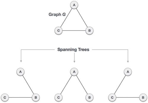
A spanning tree can be found using DFS or BFS and is the equivalent of finding the MST for an unweighted graph or graph where all the weights are the same.
Basically while there are cycles in the graph just keep removing an edge from the cycle until there are no more cycles.
Now let’s define the total weight of a graph as the sum of the weights of all of the edges in the graph. More formally:
\[\text{weight}(G) = \sum_{e \in E} w(e) \]Where \(E\) is the set of all edges in the graph and \(w(e)\) is the weight of the edge \(e\). The company now wants to optimize the cost of sending their employees to all of the capitals in Europe. So what they want is to find the spanning tree with the minimum total weight. This is called the minimum spanning tree (MST) problem. This example for the problem only works if we assume all cities are equally important, otherwise we would obviously analyze which capital is visited the most and then optimize the route based on that.
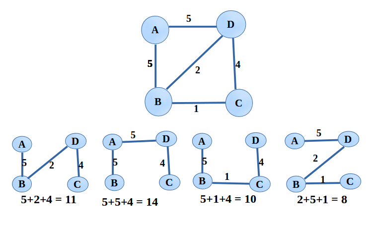
Notice that all spanning trees have the same number of edges, \(|V| - 1\), where \(|V|\) is the number of vertices in the graph. This is because a tree with \(|V|\) vertices has \(|V| - 1\) edges if there were more edges then there would be a cycle in the graph and if there were fewer edges then the graph would not be connected or there would be a vertex that is not reachable.
In this example negative weights anyway do not make sense as the cost of a flight can not be negative. But in general, the weights of the edges can be negative, and will not change the problem, the only thing that can happen is that the minimum spanning trees weight becomes negative. Lets look at some of the properties of minimum spanning trees.
Cycle Property
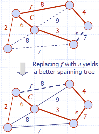
The cycle property is very simple, if you have a cycle in the original graph \(G\) and you have an edge \(e\) with the maximum weight in that cycle, then \(e\) can not be part of the minimum spanning tree. The reason and proof for this is relatively simple. Let’s assume that \(e\) is part of the minimum spanning tree, then because \(e\) can be replaced by any other edge in the cycle, the total weight of the minimum spanning tree would decrease. This is a contradiction because we assumed that the minimum spanning tree was the minimum spanning tree.
Uniqueness
When calculating the minimum spanning tree of a graph there can be multiple valid solutions as we can see in the example below. This is due to the fact that some of the edges in the graph have the same weight. However, just because the weights are not unique does not mean that the minimum spanning tree is not unique. If all the weights in an MST solution are smaller than the weights of the other edges, then the MST is unique as these edges would not make the tree any lighter. An obvious example is given an MST you add lots of edges that are the same weight but heavier than the heaviest edge in the MST, then the MST is still the same.
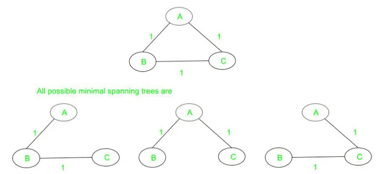
However, if all the edges in the graph have a unique weight, then the minimum spanning tree is unique.
todo show that there are two edges that must have the same weight because of the cycle property
Cut Property
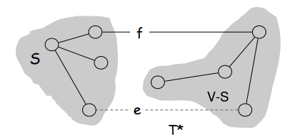
The goal of the cut property is to show which edges are guaranteed to be part of the minimum spanning tree, also called safe or light edges. A cut of a graph is a partition of the vertices into two disjoint sets, \(S\) and \(T\) where \(S \cup T = V\) and \(S \cap T = \emptyset\) and \(S \neq \emptyset\) and \(T \neq \emptyset\). An edge is said to cross the cut if one of its endpoints is in \(S\) and the other is in \(T\). The cut-set of a cut is the set of edges that cross the cut.
So you can think of a cut as a way to divide the graph into two parts, so all the capital cities in western Europe are in \(S\) and all the capital cities in eastern Europe are in \(T\). The cut-set is then the set of all the flights between the two parts of Europe.
The cut property then states that for all cuts of a graph, the minimum weight edge crossing the cut is part of the minimum spanning tree. This is a very intuitive property, as the minimum spanning trees goal is to connect all the vertices in the graph with the smallest total weight. If we have a cut that separates the graph into two parts, then the minimum weight edge crossing the cut is the lightest way to connect the two parts of the graph.
Minimum-cost Edge Property
The minimum-cost edge is like a special case of the cut property. It states that the edge with the minimum weight i.e cost is always part of the minimum spanning tree. This is a very intuitive property, as the minimum spanning tree is the tree with the smallest total weight, so the lightest edge in the graph must be part of the minimum spanning tree.
The proof is also very obvious. If \(e\) is the minimum cost edge in the graph, then the minimum spanning tree must contain \(e\). There is no lighter way to connect the two vertices of \(e\). If all the edges have different weights and \(e\) is not part of the MST, then the MST would not be the minimum spanning tree as we could replace the edge with \(e\) and get a lighter tree.
Boruvka’s Algorithm
In 1926 a Czech mathematician called Otakar Boruvka was tasked with finding the minimum spanning tree of a graph. It was meant to help with the design and construction of the power grid in Moravia. So the graph contained houses and the power stations and the edges were the power lines between the houses and the power stations and the associated cost of building the power lines. Note that power lines can go from a house to a power station or from a house to a house. The goal was to find the minimum cost of building the power lines to connect all the houses to power.
Boruvka’s algorithm is a greedy algorithm in the sense that at each step it chooses the locally optimal solution to find the global optimal solution. The idea of the algorithm is to make use of the cut property by starting of with each vertex as a seperate component and then iteratively merging the components by adding the minimum cost edge that crosses the cut between the components. The algorithm then continues until there is only one component left, which is the minimum spanning tree.
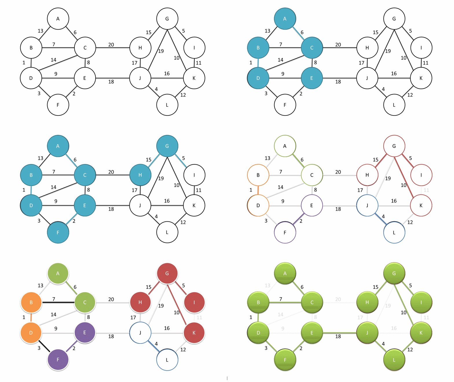
Boruvka(G):
    MST = empty set
    (C_1, C_2, ..., C_n) = all the vertices in G as seperate components
    while number of components > 1:
        for each component C_i:
            find the minimum cost edge e_i that crosses the cut between C_i and the other components
        add all the edges e_i to the MST
        merge the components that are connected by the edges e_i
    return MST
The time complexity of Boruvka’s algorithm is \(O((|V| + |E|) \log |V|)\). The outer iteration of the algorithm runs at most \(\log |V|\) times. This is because in the beginning there are \(|V|\) components and at each iteration the number of components is at least halved. This is because in the worst case each two components will pick the same edge to be merged. The inner iteration needs to look at all the edges in the graph, but also updating the components after merging processes all vertices which is where the \(O(|V| + |E|)\) comes from. Because the original graph is at least connected \(|E| \geq |V| - 1\) so the number of edges dominates the number of vertices which is why the time complexity is also often written as \(O(|E| \log |V|)\).
write the code all implementations seem to use union find, I also can’t think of a way to implement it without union find that is efficient
Prim’s Algorithm
Prim’s algorithm is another greedy algorithm that rather than merging components using the cut property, it slowly grows out the minimum spanning tree by only concentrating on a single connected component. The algorithm starts with a single vertex and then iteratively adds the minimum cost edge that connects the tree to a vertex not in the tree. The algorithm continues until all the vertices are in the tree.
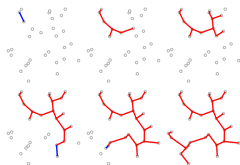
We can quickly come up with a naive implementation of Prim’s that at each step looks at all the edges and picks the minimum cost edge that connects the tree to a vertex not in the tree. This would have a time complexity of \(O(nm)\) where \(n\) is the number of vertices and \(m\) is the number of edges. If the graph is complete then \(m \in O(n^2)\) and the time complexity becomes \(O(n^3)\) which is not very efficient.
Prim(G, s):
    MST = empty set
    S = {start vertex s}
    while S != V:
        for each vertex v in S:
            find the minimum cost edge e that connects v to a vertex u not in S
        add the edge e to the MST
        add the vertex u connected by e to S
We can improve the time complexity of Prim’s algorithm by using a priority queue to improve the time of finding the minimum cost edge. The implementation then becomes very similar to Dijkstra’s algorithm as we are keeping track of the minimum cost edge to each vertex. The time complexity then \(O((|V| + |E|) \log |V|)\) which is the same as Boruvka’s algorithm after making the same assumptions for the number of edges to be \(|E| \geq |V| - 1\) and therefore \(O(|E| \log |V|)\).
Prim(G, s):
    MST = empty set
    S = {start vertex s}
    Q = priority queue with all the vertices in G and distances set to infinity
    d[s] = 0, d[v] = infinity for all other vertices
    Q.update(s, 0)
    while S != V:
        v = Q.pop()
        S = S union {v}
        add the shortest edge from v to a vertex in S to the MST
        for each vertex u connected to v where u is not in S:
            d[u] = min(d[u], w(v, u))
            Q.update(u, d[u])
The problem with the above code is finding out which edge to add to the MST efficiently to get the total weight is easy but finding the edge needs proper bookkeeping.
Kruskal’s Algorithm
Kruskal’s algorithm is another greedy algorithm that is very similar to Boruvka’s algorithm. The algorithm again makes use of the cut property but picks the edges slightly different. Rather than starting with each vertex as a seperate component and then iterating over the components and picking the minimum cost edge that crosses the cut, Kruskal’s algorithm again starts with each vertex as a seperate component but then sorts all the edges by weight and then iterates over the edges and picks the minimum cost edge that do not create a cycle which is the same as making sure the edges connect two different components. The algorithm continues until there is only one component left, which is the minimum spanning tree. The aglorithm is rather simple and can be implemented in \(O(nm)\) time where \(n\) is the number of vertices and \(m\) is the number of edges.
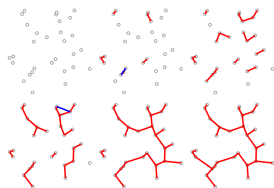
Kruskal(G):
    MST = empty set
    sort all the edges in G by weight
    (C_1, C_2, ..., C_n) = all the vertices in G as seperate components
    for each edge e from u to v in the sorted edges:
        if u and v are in different components:
            add e to the MST
            merge the components that contain u and v
The time of the above algorithm is \(O(nm)\) where \(n\) is the number of vertices and \(m\) is the number of edges. The reason for this is that the algorithm needs to sort all the edges which takes \(O(m \log m)\) time and then iterate over all the edges and then find out if the vertices are in the same component and then merge the components which takes \(O(n+m)\) time with a DFS. The time complexity can be improved by using a union-find data structure to keep track of the components and then the time complexity becomes \(O((|V| + |E|) \log |V|)\) or again \(O(|E| \log |V|)\).
Kruskal(G):
    MST = empty set
    sort all the edges in G by weight
    UF = union-find data structure with all the vertices in G
    for each edge e from u to v in the sorted edges:
        if UF.find(u) != UF.find(v):
            add e to the MST
            UF.union(u, v)