Knapsack Problem
The knapsack problem is a very popular problem with many different variations. The basic problem is as follows:
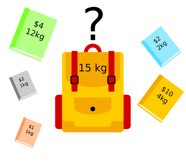
Given a set of items, each with a weight and a value, determine which items you should pick to maximize the value while keeping the overall weight smaller than the limit of your knapsack (backpack).

Some popular variations of the knapsack problem are:
- 0/1 Knapsack: You can either take an item or not take it. This is the most basic variation.
- Unbounded Knapsack: You can take an item multiple times.
- Bounded Knapsack: You can take an item a limited number of times.
- Fractional Knapsack: You can take a fraction of an item.
Some youtube videos on the knapsack problem are available:
The subset sum problem is a variation of the knapsack problem where the weight of each item is equal to its value and the goal is not to maximize the value but to get a specific value and weight.
For now let’s focus on the 0/1 knapsack problem. The 0/1 knapsack problem is the most basic variation of the knapsack problem. In this variation, you can either take an item or not take it. So we can formally define the problem as:
\[\begin{align*} \sum_{i \in I} w_i &\leq W \text{ (total weight of items in the knapsack is less than or equal to the weight limit)} \\ \sum_{i \in I} p_i &\text{ is maximized (total value of items in the knapsack is maximized)} \end{align*} \]Given a weightlimit \(W\) and a set of \(n\) items, each with a weight \(w_i \in \mathbb{N}\) and a value \(p_i \in \mathbb{N}\) for \(i \in [1, n]\), find the subset of items \(I\) so that the following conditions are satisfied:
The most naive solution to this problem is to try all possible subsets of items and check which one satisfies the weight limit and has the maximum value. However, there are \(2^n\) possible subsets of items, so this approach would take exponential time of \(O(2^n)\). So we need a more efficient solution.
We can perform some initial pruning by removing items that have a weight greater than the weight limit. This would reduce the number of items we have to consider and only costs us \(O(n)\) time. However, we still have to consider all possible subsets of the remaining items. This also results in the fact that the maximum value of the optimal solution is at least the value of the item with the highest value, as all the remaining items after the pruning can be taken:
\[\sum_{i \in OPT} p_i \geq p_{\text{max}} \]This also leads to the following upper bound on the maximum value of the optimal solution:
\[\sum_{i \in OPT} p_i \leq \sum_{i=1}^n p_i \leq n \cdot p_{\text{max}} \]Greedy Approach
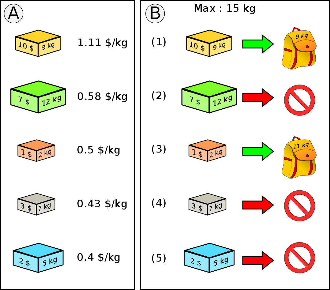
The most intuitive approach to a person is most likely to take the item with the highest value to weight ratio. This is a greedy approach which makes sense as we humans tend to be greedy. The formal definition of a greedy algorithm is that at each step, we make the locally optimal choice in the hope that it will lead to a globally optimal solution. However, these algorithms do not always work.
In the case of the knapsack problem, we could come up with a few greedy approaches:
- To always take the item with the highest value.
- To always take the item with the lowest weight.
- To always take the item with the highest value to weight ratio.

However, for all of these greedy approaches, there are counterexamples where the greedy approach does not lead to the optimal solution.
Consider the following items:
| Item | Weight | Value |
|---|---|---|
| \(1\) | \(1\) | \(1\) |
| \(\vdots\) | \(\vdots\) | \(\vdots\) |
| \(W\) | \(1\) | \(1\) |
| \(W+1\) | \(W\) | \(2\) |
If the weight limit is \(W\), the optimal solution is to take the \(W\) items with weight 1 and value 1 adding up to a total value of \(W\). The greedy strategy of taking the item with the highest value would’ve failed in this case as it would’ve taken the item with weight \(W\) and value 2.
Consider the following items:
| Item | Weight | Value | Value/Weight |
|---|---|---|---|
| \(1\) | \(1\) | \(1\) | \(1\) |
| \(2\) | \(W\) | \(W-1\) | \(1-\frac{1}{W}\) |
If the weight limit is \(W\), the optimal solution is to just take the second item with weight \(W\) and value \(W-1\). The greedy strategy of taking the lightest item would’ve failed in this case as it would’ve taken the first item with weight 1 and value 1. The same goes for the greedy strategy of taking the item with the highest value to weight ratio.
Dynamic Programming Approach
Instead of trying all possible subsets we can use dynamic programming approach just like in the subset sum problem. A possible subproblem that we could define is for all items \(i \in [1, n]\), all weights \(w \in [1, W]\) and all values \(p \in [1, P]\) where \(P\) is the sum of all values of the items. We could define the subproblem as:
\[T(i, w, p) = \begin{cases} 1 & \text{if there is a subset of items $I$ with total weight $w$ and total value $p$} \\ 0 & \text{otherwise} \end{cases} \]This would result in a 3D table of size \(n \times W \times P\) and a time complexity of \(O(n \cdot W \cdot P)\). However, we can very quickly see that this is not efficient as for example for a fixed \(i\) and \(w\) we are calculating all possible values \(p\) which is not necessary. Instead we only want to know what the maximum value is for a fixed \(i\) and \(w\).
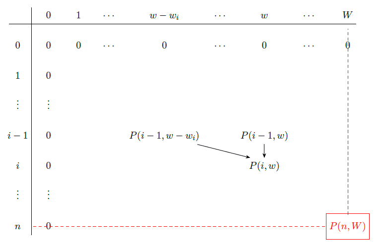
So if we want to calculate the maximum value for a fixed \(i\) and \(w\) so \(P(i, w)\) then there are two possibilities for the \(i\)-th item:
- The subset of items \(I\) does not contain the \(i\)-th item. In this case, the maximum value is the same as the maximum value for the \(i-1\) items and weight \(w\). So \(P(i, w) = P(i-1, w)\).
- The subset of items \(I\) contains the \(i\)-th item. In this case, the maximum value is the value of the \(i\)-th item plus the maximum value for the \(i-1\) items and the remaining weight \(w - w_i\). So \(P(i, w) = p_i + P(i-1, w - w_i)\).
Our base cases are when we have no items or no weight left. In this case, the maximum value is 0. So \(P(0, w) = 0\) and \(P(i, 0) = 0\) for all \(i\).
We also mustn’t forget to check if we can even take the \(i\)-th item. If the weight of the \(i\)-th item is greater than the remaining weight \(w\) then we can’t take the \(i\)-th item. So the final recursive formula is:
\[P(i, w) = \begin{cases} P(i-1, w) & \text{if $w_i > w$} \\ \max(P(i-1, w), p_i + P(i-1, w - w_i)) & \text{otherwise} \end{cases} \]public int maxProfit(int[] weights, int[] values, int weightLimit) {
int n = weights.length;
int[][] dp = new int[n + 1][weightLimit + 1];
for (int i = 1; i <= n; i++) {
for (int w = 1; w <= weightLimit; w++) {
// we can't take the i-th item
if (weights[i - 1] > w) {
dp[i][w] = dp[i - 1][w];
} else {
// is it better to take the i-th item or not
dp[i][w] = Math.max(dp[i - 1][w], values[i - 1] + dp[i - 1][w - weights[i - 1]]);
}
}
}
return dp[n][weightLimit];
}
This results in a 2D table of size \(n \times W\) and a time complexity of \(O(n \cdot W)\). Just like in the subset sum problem this is a pseudo-polynomial time complexity as it doesn’t just depend on the number of items \(n\) but also on the weight limit \(W\). We can also change the variable we are focusing on from the profit to the weight. In this case, we would have a 2D table of size \(n \times P\) and a time complexity of \(O(n \cdot P)\). Which would again be a pseudo-polynomial time complexity. Depending on the values of the items and the weight limit one of the two approaches might be more efficient.
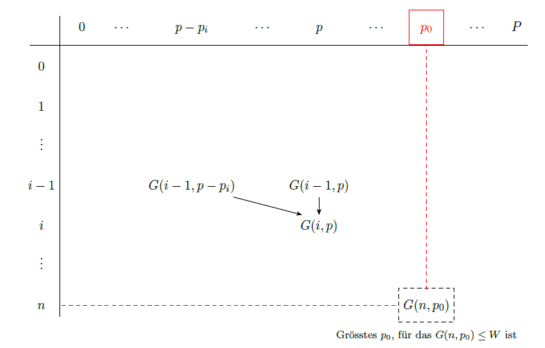
So rather then storing the maximum value that can be achieved for a fixed \(i\) and \(w\) we can also store the minimum weight that can be achieved for a fixed \(i\) and \(p\). So for a fixed \(i\) and \(p\) we have two possibilities:
- The subset of items \(I\) does not contain the \(i\)-th item. In this case, the minimum weight is the same as the minimum weight for the \(i-1\) items and value \(p\). So \(G(i, p) = G(i-1, p)\).
- The subset of items \(I\) contains the \(i\)-th item. In this case, the minimum weight is the weight of the \(i\)-th item plus the minimum weight for the \(i-1\) items to achieve the remaining value \(p - p_i\). So \(G(i, p) = w_i + G(i-1, p - p_i)\). If \(p \geq p_i\) then we have already calculated \(G(i-1, p - p_i)\). If \(p < p_i\) then just the item \(i\) is enough to achieve the value \(p\), we can cover this case by setting \(G(i-1, p - p_i) = 0\) if \(p < p_i\). So the final recursive formula is:
Our base cases are \(G(0,0) = 0\) and \(G(0, p) = \infty\) for all \(p > 0\) as we can’t achieve a positive value with no items.
public int maxProfit(int[] weights, int[] values, int value) {
    int n = weights.length;
    int sum = 0;
    for (int v : values) {
        sum += v;
    }

    int[][] dp = new int[n + 1][sum + 1];

    // base case
    for (int p = 1; p <= sum; p++) {
        dp[0][p] = Integer.MAX_VALUE;
    }

    for (int i = 1; i <= n; i++) {
        for (int p = 0; p <= sum; p++) {
            if (values[i - 1] > p) {
                dp[i][p] = Math.min(dp[i - 1][p], weights[i - 1]);
            } else {
                dp[i][p] = Math.min(dp[i - 1][p], weights[i - 1] + dp[i - 1][p - values[i - 1]]);
            }
        }
    }

    // extract maximum value
    int maxProfit = 0;
    for (int p = 0; p <= sum; p++) {
        if (dp[n][p] <= value) {
            maxProfit = p;
        }
    }

    return maxProfit;
}
Knapsack for P vs NP
Knapsack and subset sum are both NP-complete problems so they can be reduced to each other or also to other NP-complete problems such as SAT. So solving one of these pseudo-polynomial time complexity problems in polynomial time would mean that P=NP.
Approximative Approach
Because we can’t calculate the optimal solution in polynomial time we can try to find an approximative solution. The idea of one approximative algorithm is to reduce the number of values we are considering. In the approach where each entry contains the minimum weight to achieve a certain value we are considering all possible values, resulting in a time complexity of \(O(n \cdot P)\). We want to reduce the number of values we are considering. We can do this by rounding the values of the items. So we pick some factor \(k\) and round the values of the items down to the nearest multiple of \(k\):
\[\hat{p}_i = k \cdot \left\lfloor \frac{p_i}{k} \right\rfloor \]So for example if we have \(k=10\) and \((p_1, p_2, p_3, p_4) = (112, 78, 1001, 237)\) then \((\hat{p}_1, \hat{p}_2, \hat{p}_3, \hat{p}_4) = (110, 70, 1000, 230)\). So now instead of having to look at all \(P\) columns we only have to look at each \(k\)-th column, or we can also reduce the number of columns by a factor of \(k\) and have a table of size \(n \times \frac{P}{k}\). This results in a time complexity of \(O(n \cdot \frac{P}{k})\).
The question now is how good of an approximation this is. For this we can make a few observations:
- The actual values of the items don’t change by that much as \(\hat{p}_i \leq p_i \leq \hat{p}_i + k\).
- Because the algorithm only changes the values of the items and not the weights they both still cover the same subsets of items. The only difference is that due to the rounding the value of the subset might be slightly different. This means that every subset produced by the approximative algorithm is a valid solution for the original problem but not necessarily the optimal solution.
If we define the subset produced by the optimal algorithm as \(OPT\) and the subset produced by the approximative algorithm as \(\overline{OPT}\) then the question remains how good of an approximation \(\overline{OPT}\) is to \(OPT\). We denote the maximum value as \(p(OPT)\) and \(p(\overline{OPT})\) as:
\[P(OPT) = \sum_{i \in OPT} p_i \quad \text{and} \quad P(\overline{OPT}) = \sum_{i \in \overline{OPT}} p_i \]Because both optimal solution and approximative solution cover the same subsets of items we have for all possible subsets \(I\) that fit in the knapsack:
\[\sum_{i \in \overline{OPT}} \hat{p}_i \geq \sum_{i \in I} \hat{p}_i \]This also counts for \(I=OPT\) as \(OPT\) is a valid subset of items that fit in the knapsack. This means that:
\[\sum_{i \in \overline{OPT}} \hat{p}_i \geq \sum_{i \in OPT} \hat{p}_i \]So if we slowly combine all our observations from above we get:
\[\begin{align*} P(\overline{OPT}) &= \sum_{i \in \overline{OPT}} p_i \\ &\geq \sum_{i \in \overline{OPT}} \hat{p}_i \\ &\geq \sum_{i \in OPT} (p_i - k) \\ &= P(OPT) - |OPT| \cdot k \\ &\geq P(OPT) - nk \\ &\geq P(OPT) - nk \cdot \frac{P(OPT)}{p_{\text{max}}} \\ &= P(OPT) \left(1 - \frac{nk}{p_{\text{max}}} \right) \\ &= P(OPT) \left(1 - \epsilon \right) \\ &= P(OPT) - \epsilon \cdot P(OPT) \end{align*} \]So depending on the factor \(k\) we can get a better or worse approximation. With the approximative algorithm we can get an approximation of the optimal solution that is at least \((1 - \epsilon)\) times the optimal solution. We now want to minimize the error \(\epsilon\) to get the best approximation. By reformulating the error we get:
\[k = \frac{\epsilon \cdot p_{\text{max}}}{n} \]So if we have \(n=10\) items and \(p_{\text{max}}=1000\) then if we want to have an error of \(\epsilon=0.1\) so the approximative algorithm produces a maximum value that is at least \(0.90\) times the optimal value we would have to round the values of the items to the nearest multiple of \(10\).
\[k = \frac{0.1 \cdot 1000}{10} = 10 \]We can also see how the error \(\epsilon\) affects the time complexity. The time complexity of the approximative algorithm is \(O(n \cdot \frac{P}{k})\) which results in:
\[\begin{align*} O(n \cdot \frac{P}{k}) &= O(n \cdot \frac{P}{\frac{\epsilon \cdot p_{\text{max}}}{n}}) \\ &= O(nP \cdot \frac{n}{\epsilon \cdot p_{\text{max}}}) \\ &= O(n^2 \cdot \frac{P}{\epsilon \cdot p_{\text{max}}}) \\ &= O(\frac{n^3}{\epsilon}) = O(n^3) \end{align*} \]The last parts coming from the fact that \(P \leq n \cdot p_{\text{max}}\) and that \(epsilon > 0\) is a constant. Due to this the approximative algorithm is a so called polynomial time approximation scheme (PTAS) as we can calculate an \((1 - \epsilon)\) approximation in polynomial time.
We can also set \(\epsilon = \frac{1}{n}\) so making it dependent on the number of items. This results in a time complexity of \(O(n^4)\) and makes the approximative algorithm a fully polynomial time approximation scheme (FPTAS).