Shortest Path Algorithms

The diameter of a graph is the longest shortest path between two vertices in the graph. So in the above example, the diameter of the graph is 3 as the longest shortest path is between Michael and Karen.

• diameter
• BFS
• Dijkstra’s algorithm
• Bellman-Ford algorithm
• A* algorithm

One of the most known problems in graph theory is the shortest path problem. The problem is to find the shortest path between two vertices \(u\) and \(v\) in a graph. Depending on the type of graph the definition of shortest path can vary.

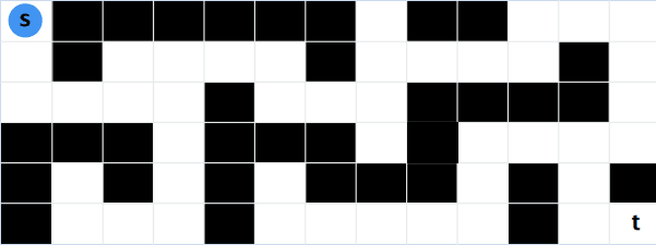
Unweighted Graphs

In an unweighted graph, the shortest path is the path with the fewest number of edges. This would be the same as if we would give all edge the weight of 1 or just the same positive weight.

To solve this problem we can simply use the Breadth First Search (BFS) algorithm. As with BFs we start at the source vertex \(s\) and visit all the vertices that are at distance 1 from \(s\) if we haven’t found our target vertex \(t\) we go to the next level and visit all the vertices that are at distance 2 from \(s\) and so on. Once we have found the target vertex we know that the shortest path has been found and we can stop the algorithm. To be able to reconstruct the path we also have to store from which node we came to the current node.

public List<Integer> shortestPath(List<List<Integer>> graph, int start, int target) {
   boolean[] visited = new boolean[graph.size()];
   // store from which node we came to the current node
   int[] parent = new int[graph.size()];
   Arrays.fill(parent, -1);
   Queue<Integer> queue = new LinkedList<>();
   queue.add(start);
   visited[start] = true;
   while (!queue.isEmpty()) {
      int node = queue.poll();
      if (node == target) {
         break;
      }
      for (int neighbor : graph.get(node)) {
         if (!visited[neighbor]) {
               visited[neighbor] = true;
               parent[neighbor] = node;
               queue.add(neighbor);
         }
      }
   }
 
   // couldn't find the target
   if (parent[target] == -1) {
      return Collections.emptyList();
   }
 
   // reconstruct the path
   List<Integer> path = new ArrayList<>();
   for (int at = target; at != -1; at = parent[at]) {
      path.add(at);
   }
   Collections.reverse(path);
   return path;
}

We know that the time complexity of BFS is \(O(m + n)\) where \(m\) is the number of edges and \(n\) is the number of vertices. This algorithm also shows that the time complexity of finding the shortest path between two vertices or the shortest path to all vertices from a single vertex is the same as in the worst case we have to visit all vertices and edges in the graph. This is why when we talk about the shortest path problem we are actually talking about the single source shortest path problem or one-to-all shortest path problem.

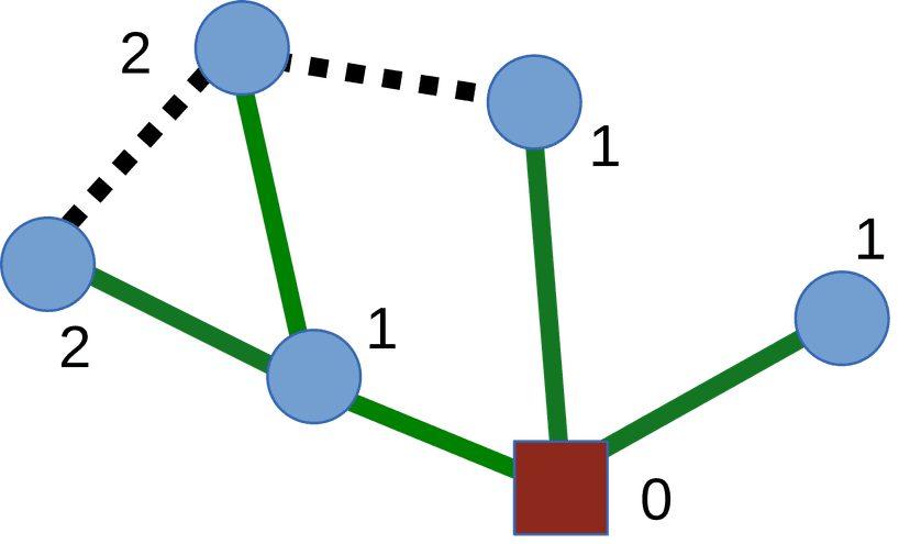
If we draw a tree where all the nodes that are at distance \(d\) from the source node \(s\) are at level \(d\) then we have a so called BFS tree or shortest path tree. The tree is rooted at the source node \(s\) and the shortest path from \(s\) to any other node in the graph is the path from \(s\) to the node in the BFS tree. The BFS tree is a subgraph of the original graph and it contains all the vertices in the graph.

We can also use the Depth First Search (DFS) algorithm to find the shortest path between two vertices in an unweighted graph. However, breadth-first search is preferred due to the possible recursion overhead of DFS. If we know that the graph is a DAG we can also use topological ordering to find the shortest path between two vertices.

Dijkstra’s Algorithm

For weighted graph, the shortest path is the path with the smallest sum of weights of the edges. For now we will assume that all the weights are positive.

There are some important properties of the shortest path problem that we should be aware of. The first one is Triangle Inequality. The triangle inequality states that the shortest path between two vertices is the direct path between the two vertices. So more formally:

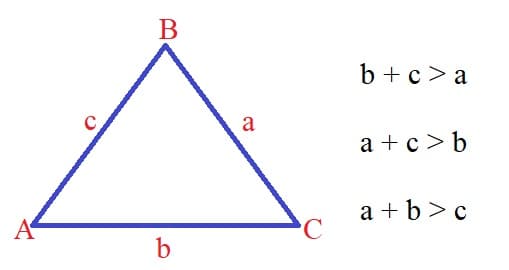
This leads to the fact that if the shortest path between two vertices is \(v_1, v_2, \ldots, v_n\) then the subpath between any two vertices \(v_i\) and \(v_j\) is also the shortest path between these two vertices. This is also why we can say that the shortest path will always be a path and not a walk as it would make no sense to visit a vertex more than once. We can also define this formally:

Or in other words:

The idea of Dijkstra’s algorithm to find the shortest path between two vertices is based on these properties. It’s a greedy algorithm that can also be seen as a dynamic program. The goal is to iterativly build up the shortest paths from the source vertex to all other vertices by finding the ideal \(v_i\) for each vertex \(v\). When it has found a \(v_i\) that is better then the previous one it updates the shortest path to the vertex \(v\), this process is also called relaxation. However, when doing so we want to be sure that \(\text{d}(u, v_i)\) is already the final solution so we need to bring some sort of order into our dynamic program. We do this we sorting the vertices by their distance to the source vertex. This is why we use a priority queue to store the vertices and always take the vertex with the smallest distance to the source vertex and then relax all the edges that go out from this vertex.

public int[] dijkstra(List<List<Integer>> graph, List<List<Integer>> weights, int start) {
   int[] dist = new int[graph.size()];
   Arrays.fill(dist, Integer.MAX_VALUE);
   dist[start] = 0;
   // store the vertex and its current minimum distance to the source vertex
   PriorityQueue<Pair>> pq = new PriorityQueue<>(Comparator.comparingInt(p -> p.second));
   pq.decreaseKey(start, 0);
   while (!pq.isEmpty()) {
      Pair<Integer, Integer> pair = pq.poll();
      int node = pair.first;
      int distance = pair.second;
      
      for (int i = 0; i < graph.get(node).size(); i++) {
         int neighbor = graph.get(node).get(i);
         int weight = weights.get(node).get(i);
         // relax neighbors
         if (dist[node] + weight < dist[neighbor]) {
            dist[neighbor] = dist[node] + weight;
            pq.decreaseKey(neighbor, dist[neighbor]);
         }
      }
   }
   return dist;
}

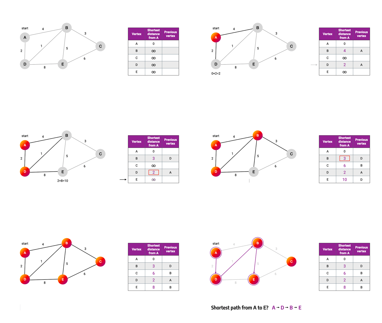
The time complexity of Dijkstra’s algorithm is \(O((m+n) \log n)\) where \(m\) is the number of edges and \(n\) is the number of vertices. The reason for this is that the minimum is extracted \(n\) times and the decreaseKey operations is called \(m\) times which both have a time complexity of \(O(\log n)\). If a Fibonacci heap is used as the priority queue the time complexity of Dijkstra’s algorithm changes from \(O((m+n) \log n)\) to \(O(m + n \log n)\).

However at the moment I have no idea how a Fibonacci heap works.

Now what if we used Dijkstra’s algorithm on a graph with negative weights. Then the properties mentioned above such as the triangle inequality on which the algorithm is based on would not hold. This is why Dijkstra’s algorithm can only be used on graphs with non-negative weights.

Bellman-Ford Algorithm

The Bellman-Ford algorithm is another algorithm that can be used to find the shortest path between a source vertex and all other vertices in a graph. It is slower than Dijkstra’s algorithm with a time complexity of \(O(mn)\) where \(m\) is the number of edges and \(n\) is the number of vertices. However, unlike Dijkstra’s algorithm, the Bellman-Ford algorithm can handle graphs with negative weights. The key problem with Dijkstra’s algorithm and why it can not handle negative weights is that it doesn’t revist a vertex after it has been relaxed. So if a shorter path exists through a a longer path with negative weights the algorithm will not find it.

The only restriction is that the graph can not contain negative cycles, so a cycle where the sum of the weights is negative. The reason for this is that if there is a negative cycle in the graph then there is no shortest path between the vertices in the graph as we can just repeatedly traverse the cycle and get a shorter path each time. However, the Bellman-Ford algorithm will detect if there is a negative cycle in the graph and return that there is no shortest path between the vertices in the graph.

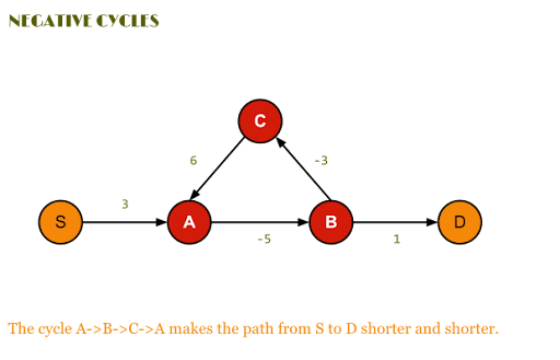
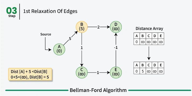
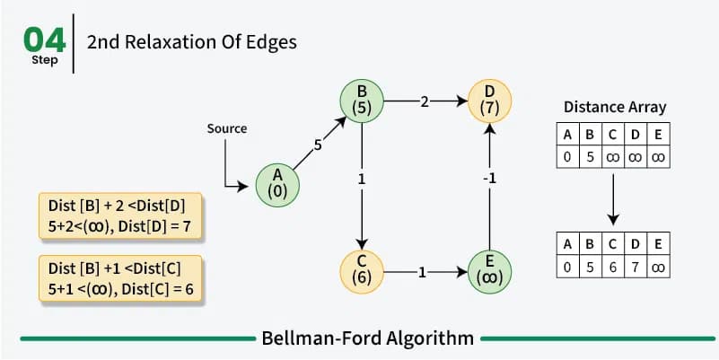
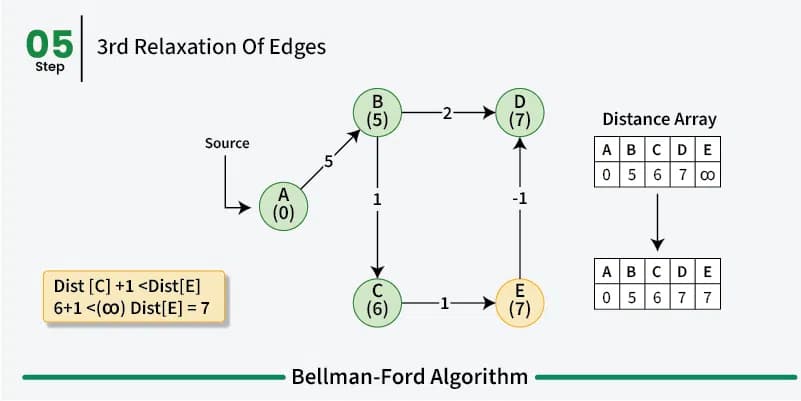
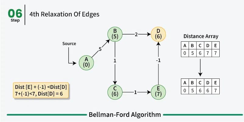
Bellman-Ford is just like Dijkstra’s algorithm a greedy dynamic programm and works in a similar way by relaxing the distances to the start vertex. However, rather then using a priority queue to pick the vertex with the smallest distance to the start vertex and then relaxing all its neighbors, the Bellman-Ford algorithm relaxes all the edges in the graph \(n-1\) times.

So we iterate \(n-1\) times over all the edges in the graph and look at the end points of the edges. So if we have an edge from \(u\) to \(v\) with weight \(w\) we relax the distance to \(v\) by adding the weight of the edge to the distance to \(u\). This way we can be sure that we have found the shortest path between the vertices in the graph. In the first iteration we only know that we can reach the start vertex with a distance of 0. All other vertices have a distance of infinity. In the second iteration we know that we can reach all the vertices that are directly connected to the start vertex with the weight of the edge between the two vertices and so on.

As already mentioned before a shortest path between two vertices can have at most \(n-1\) edges as walk doesn’t make sense. So after \(n-1\) iterations all the shortest paths have been found. We do these multiple iterations for the possibility of negative weight in the graph making previous paths shorter. If we do a \(n\)th iteration and we find that we can still relax the distances then we know that there is a negative cycle in the graph.

The time complexity of the Bellman-Ford algorithm is \(O(mn)\) because we iterate over all the edges \(n\) times.

public int[] bellmanFord(List<List<Integer>> graph, List<List<Integer>> weights, int start) {
   int[] dist = new int[graph.size()];
   Arrays.fill(dist, Integer.MAX_VALUE);
   dist[start] = 0;
   for (int i = 0; i < graph.size() - 1; i++) {
      // relax all edges
      for (int u = 0; u < graph.size(); u++) {
         for (int j = 0; j < graph.get(u).size(); j++) {
            int v = graph.get(u).get(j);
            int weight = weights.get(u).get(j);
            // relax edge
            if (dist[u] + weight < dist[v]) {
               dist[v] = dist[u] + weight;
            }
         }
      }
   }
   // check for negative cycles
   for (int u = 0; u < graph.size(); u++) {
      for (int j = 0; j < graph.get(u).size(); j++) {
         int v = graph.get(u).get(j);
         int weight = weights.get(u).get(j);
         if (dist[u] + weight < dist[v]) {
            // we would relax the distance again so there is a negative cycle
            return new int[0];
         }
      }
   }
   return dist;
}

graphsBellmanFordFirstRelax.png