Communities
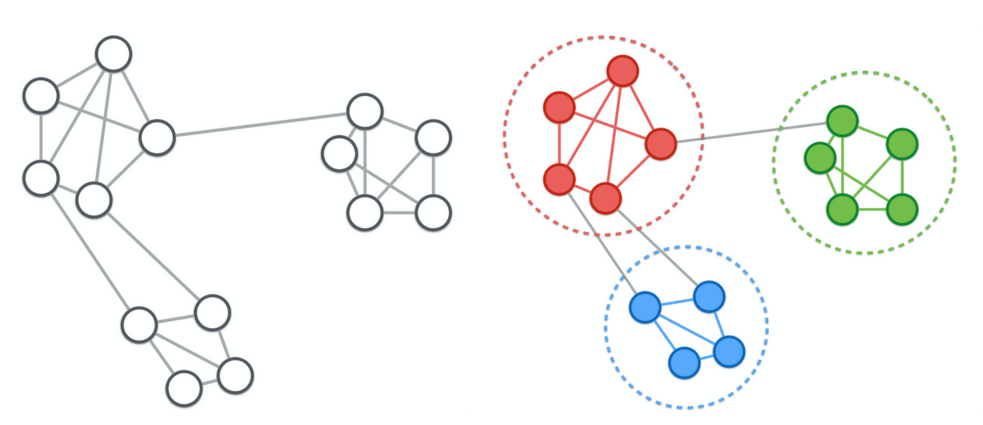
Communities are subgraphs (subsets or groups of vertices of the original graph), that are better connected to each other than to the rest of the graph. Communities are very important when analyzing social networks and networks in general as they often form around a context or a topic such as family, friends, work, hobbies, etc.
These communities can then be further analyzed such as to find out who are the most important people in a community, what is there impact on the community, and how do they relate to other communities.
Neighborhoods
The neighborhood of a vertex is the set of all vertices that are connected to by an edge, and is denoted by or if the graph is not ambiguous. The neighborhood of a vertex is also sometimes referred to as the open neighborhood when it does not include the vertex itself , and the closed neighborhood when it does include the vertex itself. The default is the open neighborhood, whereas the closed neighborhood is denoted by or .
For the given Graph and the vertex , the neighborhood is the set of vertices .
Connected Components
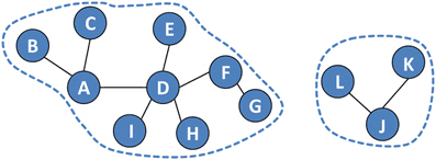
Simply put a connected component is a subgraph of the original graph where all vertices are connected to each other. So There are no disconnected vertices in a connected component. These can quiet easily be seen by eye but the definition can become more complex when we look at directed graphs.
Undirected Graphs
In an undirected graph, a connected component is a subset of vertices such that there is a path between every pair of vertices in the subset. In other words, a connected component is a subgraph of the original graph where all vertices are connected to each other.
This could be useful for example to find out if a graph is fully connected or not. If the graph has only one connected component, then it is fully connected. If it has more than one connected component, then it is not fully connected.
If we think of a communication network, then a connected component would be a group of people that can communicate with each other. If there are multiple connected components, then there are groups of people that cannot communicate with each other.
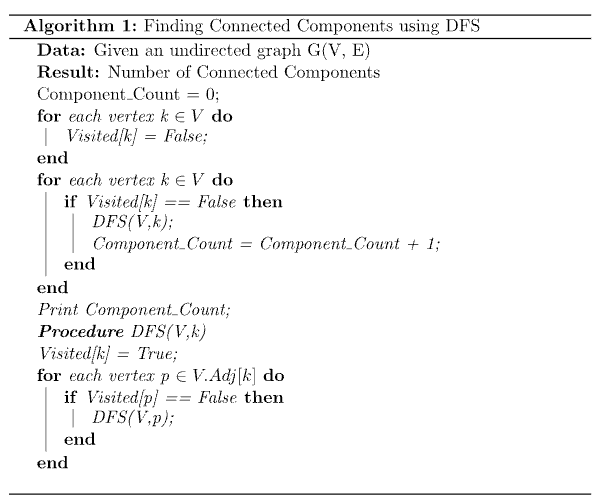
To find the connected components of a graph, we can simply use either a breadth-first search or a depth-first search over all vertices. The algorithm would then look something like this:
Directed Graphs
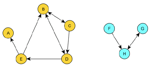
In a directed graph the directions of the edges matter. This gives us two types of connected components, weakly connected components and strongly connected components.
Weakly Connected Components
Weakly connected components are the same as connected components in an undirected graphs. So you just ignore the directions of the edges.
Strongly Connected Components
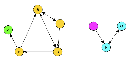
Strongly connected components are a bit more complex. In a directed graph, a strongly connected component is a subset of vertices such that there is a path between every pair of vertices in the subset, but the path must follow the direction of the edges.
Giant Components
If a connected component includes a large portion of the graph, then it is commonly referred to as a "giant component". There is no strict definition of what a giant component is, but it is commonly used to refer to connected components that include more than 50% of the vertices in the graph.
Cliques
Cliques focus on undirected graphs. A clique is a complete subgraph of the original graph, i.e a subgraph where all vertices are connected to each other. Cliques are very important in social networks as they represent groups of people that all know each other, however in a communication network they would represent a group with redundant connections.
Because cliques are complete subgraphs, they are very easy to see but also happen to be very rare and hard to find algorithmically. In the graph below the two cliques have been highlighted in red and blue.
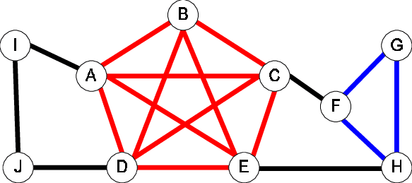
Alogrithms seem to be seperated in finding a maximal clique or finding cliques of a certain size.
Clustering Coefficient
The clustering coefficient is a metric that measures how close a graph is to being a clique (don't ask me why it isn't called Clique Coefficient). There are two different versions of the clustering coefficient, the global clustering coefficient and the local clustering coefficient, where the global clustering coefficient is just the average of the local clustering coefficients.
The idea behind the local clustering coefficient is to check how many of the neighbors of a vertex are connected to each other. If all neighbors are connected to each other, then the local clustering coefficient for that vertex is . More formally, the local clustering coefficient for a vertex is defined as:
where denotes the set of neighbors of .
For the given Graph and the vertex , the cluster coefficient is because all neighbors are connected.
For the given Graph and the vertex , the cluster coefficient is because none of the neighbors are connected.
The global clustering coefficient is then just the average of the local clustering coefficients of all vertices in the graph.
k-Core
For a k-Core the rules of a clique are slightly relaxed. A k-Core is a subgraph where all vertices are at least connected to other vertices in the subgraph.
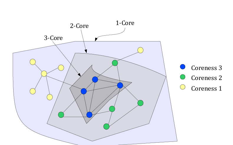
Although this is a relaxation of the rules, it is still a very strict rule and can lead to vertices that don't fulfill the connections but are only connected to other vertices in a core to not be included in the core.
Degeneracy of a graph and k-degenerate graphs is exactly this
p-Clique
The idea of a p-clique is also to relax the rules of a clique whilst also solving the above-mentioned issue of the k-core. In a p-clique, the p stands for a percentage in decimal i.e. a ratio. So in a p-clique at least the given percentage of edges of a vertices must be connected to other vertices in the subgraph.
So if we have a 0.5-clique, then at least 50% of the edges of a vertex must be connected to other vertices in the subgraph. This then allows for the vertices that don't fulfill the rule to be included in the subgraph for a k-core but are only connected to other vertices in the subgraph to be included in the subgraph.
n-Clique
Sometimes cliques are named after the number of vertices they contain. For example a clique with 3 vertices is called a 3-clique, a clique with 4 vertices is called a 4-clique, etc. this can be generalized to a k-clique. Not an n-clique though, that is something else, but when it just says 4-clique it can be ambiguous.
The idea of an n-clique is that we want a maximal subgraph, i.e. with the most vertices, where each pair of vertices can be connected by a path of length at most n. So a 1-clique is just a normal clique, a 2-clique is a clique where each pair of vertices can be connected by a path of length at most 2, etc.
The path doesn't have to be the shortest path, just a path of length at most n. And the path can go over any vertex, not just vertices that are part of the clique.
This can lead to two interesting scenarios:
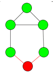
- The diameter of the subgraph can actually be longer then n. This is due to the path being able to go over any vertex, not just vertices that are part of the clique. So in the example below, the diameter of the subgraph is 3 even though it is a 2-clique.
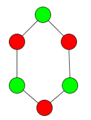
- The subgraph can be disconnected. In the example below you can see two possible 2-cliques of many for the given graph. Interestingly, they are both disconnected, because if one of the vertices inbetween is included, then a different vertex can no longer be included.
Clustering
In general clustering is the process of grouping similar objects together. In graph theory, the clustering process can be seen as a way to group vertices together i.e. to find communities that aren't based on specific rules like cliques or connected components.
There are two main approaches to clustering graphs:
- bottom-up: start with each vertex in its own cluster and then merge clusters together
- top-down: start with all vertices in one cluster and then split the cluster into smaller clusters
Girvan-Newman Clustering
The Girvan-Newman clustering algorithm is a bottom-up approach to clustering which is based on edge betweenness, hence it is also called edge betweenness clustering. The idea is to iteratively calculate the edge-betweenness of each edge in the graph and then remove the edge with the highest edge-betweenness.
The thought process behind this is that the edges with the highest edge-betweenness are the edges that have the highest information flow. So by removing these edges, we are removing the edges that connect two groups/clusters/communities together. Eventually this will lead to two components, which are then the clusters.
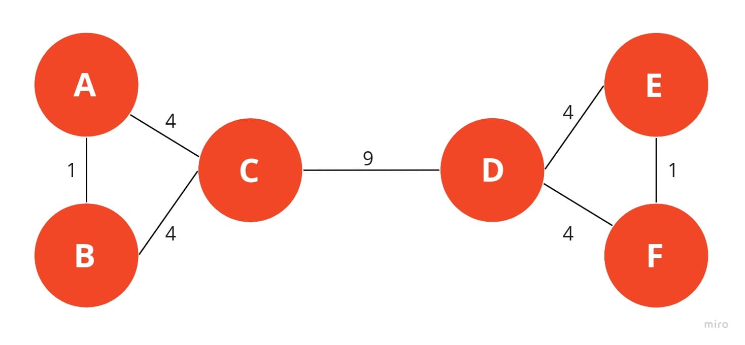
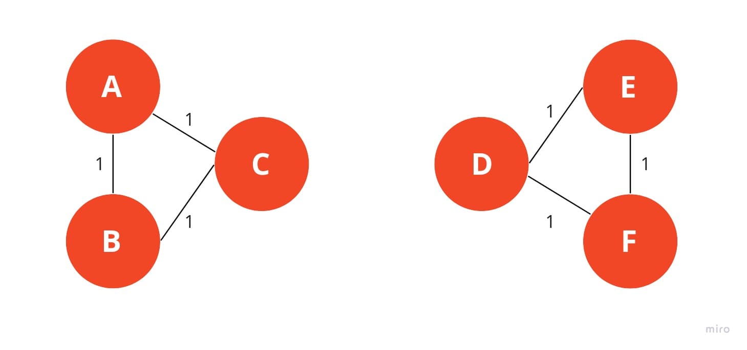
The issue with this approach is that it is very computationally expensive. The edge-betweenness of each edge has to be calculated, which is and then that has to be done iteratively multiple times so the overall complexity can be summarized to which is not ideal for large graphs.
LPA - Label Propagation Algorithm
The LPA is a more general algorithm which doesn't have to just be used for clustering graphs it can also be used to cluster data in general. However, I will explain it in the context of graph clustering.
Maybe one day this can be done in the context of semi-supervised labeling
LPA consists of 2 parts, the preparation and the actual algorithm. In the preparation we do the following:
-
We assign each vertex a unique label from to . The labels in the end will be the clusters, which makes this a bottom-up approach.
-
We perform graph coloring. I will not go into detail about graph coloring here, but the idea is to color the graph such that no two connected/neighboring vertices have the same color whilst using the least amount of colors possible.
Maybe add a link to the graph coloring chapter if it ever gets written.
Once the preparation is done, we can start the actual algorithm. The algorithm is very simple:
For each color (always in the same order) we go through each vertex (also always in the same order) and check the labels of its neighbors and count how many times each one occurs. If there is a label that occurs more often than the others, then we assign that label to the vertex. If there are multiple labels that occur the same amount of times, then there are two options:
- If the vertexes label is one of the labels that occur the most, then we keep the label.
- If the vertexes label is not one of the labels that occur the most, then we assign it the label with the highest value. Lowest would also work, as long as it is consistent.
This is repeated until the labels don't change anymore. The labels in the end then represent the clusters. The algorithm is very simple and fast making it a good choice for large graphs. However, it is not deterministic, i.e. it can lead to different results depending on the order of the colors and vertices. This can be mitigated by running the algorithm multiple times and then taking the most common result.
After the initial setup, we get the graph below:
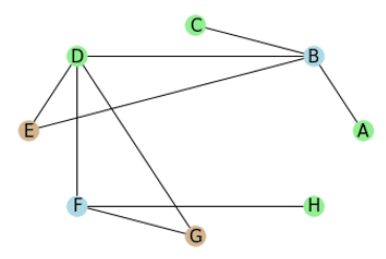
We will work through the graph in the following order:
- Blue:
- Green:
- Brown:
We start with vertex which has the neighbors with the labels . The vertex has the label . Because all the neighboring labels occur once and the vertexes label is not one of the labels we pick the one with the height value, which is . So we assign the label to .
We have a similar situation for the next vertex which gets assigned the label .
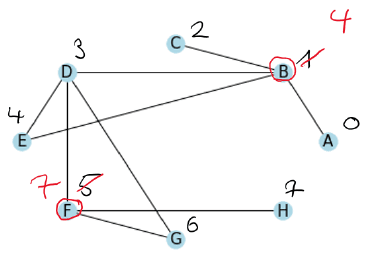
Now we do the same with the green vertices.
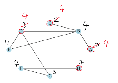
Lastly, we process the brown vertices in the given order.
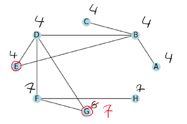
Luckily with this graph, we already have our clusters after the first iteration. We have two clusters, the vertices with the label 4 and the vertices with the label 7.
Make my own images where the graph is processed alphabetically. And what if we want more then 2 clusters?
Louvain Clustering
The Louvain clustering algorithm is a bottom-up greedy approach to clustering which is based on modularity. So we first need to understand what modularity is.
Modularity
Modularity is a metric that measures the quality of a clustering. The idea is to compare the number of edges within a cluster with the number of edges between clusters. A good clustering would then have a lot of edges within a cluster and not many edges between clusters.
Modularity is defined as the fraction of edges of a graph within a cluster minus the expected fraction of edges within a cluster if the edges were distributed randomly. The value of modularity is between and , where any value above 0 means that the number of edges within a cluster is higher than the expected number of edges within a cluster if the edges were distributed randomly. The higher the value, the better the clustering, if the value is above 0.3 then the clustering is considered to be good.
with the following definitions:
- is the weight of the edge between vertices and
- is the sum of all edge weights so for an unweighted graph and for a weighted graph .
- is the Kronecker delta function (1 if and 0 otherwise), which is used to check if two vertices are in the same cluster.
The Louvain Algorithm
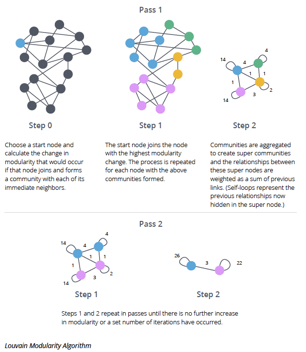
The Louvain algorithm then tries to maximize the modularity of a graph in an iterative process until the modularity cannot be increased anymore, hence it is a greedy approach.
Initially each vertex is in its own cluster. We then iteratively perform the following steps:
- Modularity Optimization: For each vertex we check how the modularity would change if we would move it to a neighboring cluster. If the modularity would increase, then we move the vertex to the neighboring cluster which would increase the modularity the most. If the modularity would not increase, then we leave the vertex in its current cluster. Once we have gone through all vertices, we move on to the next step.
- Cluster Aggregation: We then aggregate all vertices in the same cluster into a single vertex. This vertex has a self-looping edge with a weight equal to the sum of all the edges of the vertices in the cluster. The vertices resembling the clusters are then connected to each other with edges of weight equal to the sum of all the edges between the clusters before the aggregation. We then go back to the first step and repeat the process until the modularity cannot be increased anymore.
